Fixing Bottlenecks in Lead Pipe Funding: EPA’s Allotment Formula

Last fall, EPA announced that the remaining two years of Infrastructure Investment and Jobs Act allotments for lead service line replacement (IIJA–LSLR) will be based on inventory data. This shift is a positive step. However, EPA’s current allotment formula may still skew funding by disproportionately benefiting states with incomplete inventories.

In a previous blog, I outlined three key bottlenecks slowing the flow of lead service line (LSL) replacement funding. Here, I take a closer look at how EPA’s current allotment formula contributes to those delays and how it could be improved to direct funds more efficiently while strengthening incentives for inventories and replacements.

Why EPA’s Allotment Formula Falls Short

How EPA Determines LSL Allotments

After ensuring each state and territory receives its minimum allotment, EPA distributes the remaining funds via a formula based on each state’s estimated share of national LSLs (see EPIC’s IIJA LSLR allotment explainer). These state-level estimates are derived from service line material data reported by water systems. 

Because many service lines are still categorized as “unknown,” EPA estimates how many are likely to be lead by assuming unknown lines follow the same material distribution as reported lines. In other words, if 10% of reported lines are identified as lead, then 10% of unknowns are assumed to be lead. Systems with no data (i.e., unreported) were assumed to have only non-lead service lines.

Incomplete State Inventories May Be Inadvertently Rewarded

My previous analysis found that EPA’s current approach disproportionately favors states with incomplete inventories by inflating their LSL estimates. This is particularly true when a few well-inventoried water systems report high proportions of LSLs while many others report large numbers of unknowns. 

Despite progress, significant data gaps remain. Many systems still report substantial numbers of “unknown” lines, and some have not submitted inventories at all. For example, one-third of New Mexico’s systems missed the federal deadline to submit initial inventories, and New York still has more than 935,000 unidentified lines. Until these gaps are closed, EPA must rely on extrapolation for state-level LSL estimates.

Not All “Unknowns” Are Equally Likely To Be LSLs

Homes in neighborhoods built before the 1950s are far more likely to contain LSLs, while neighborhoods built after 1990 rarely do. This is because the installation of LSLs had largely phased out by the mid-1950s and was federally banned by 1986.

Importantly, the likelihood of LSLs being present also varies across states. For example, though New Mexico and Pennsylvania reported similar percentages of unknown lines (63% and 61%, respectively), differences in housing age, climate, and development patterns suggest that those unknowns are far more likely to be LSLs in Pennsylvania than in New Mexico.

Why It Matters

• Misaligned funding and needs: How EPA treats unknown service lines directly shapes state LSL estimates and, therefore, funding allocations, including the reallocation of unspent funds from prior years. EPA’s current approach can favor states with incomplete inventories, slowing the flow of funds to areas with well-documented needs. Just as importantly, it may create unintended incentives for states to delay progress on completing inventories.

• Misallocated resources: Requiring water systems serving newer neighborhoods to prove the absence of LSLs wastes time and money that could otherwise go toward actual replacements. Many utilities are already using predictive models based on factors like housing age and geography to identify where lead pipes are most likely. HUD and CDC use similar methods to identify communities at high risk of lead exposure. EPA could adopt a similar risk-based approach to direct resources where they will have the greatest impact.

Rethinking the Allotment Formula

How can EPA make LSL funding fairer and more effective? One approach is to adjust the allotment formula to account for both inventory completeness and the likelihood of LSL presence. 

Here’s what that could look like in practice:

Estimate LSLs Using Probability, Not Proportionality

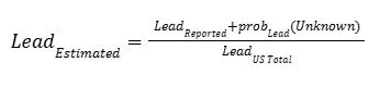
Instead of assuming unknown service lines mirror reported ones, estimate how many are likely to be lead based on their probability. This will generate more accurate state-level estimates, since not all unknowns are equally likely to be LSLs.

Penalize Incomplete Inventories

States with more complete inventories should receive a greater share of funding, while those with many unknowns should receive less. 

This can be captured by multiplying allotment amounts by a reporting rate (r):

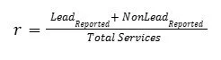
The higher the reporting rate, the more complete the inventory, and therefore the more funding directed to that state.

Fine-Tune How Strongly To Apply Penalties

This formula can be further refined to adjust how strongly these factors are weighted. For example: 

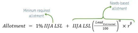
• A skewing parameter (α) shapes how funding responds to LSL estimates. When α = 1, funding is proportional to the state’s share of LSLs, but as α increases, states with higher counts receive disproportionately more funding. 

• A penalty weight (β) controls how strongly incomplete inventories are penalized. When β = 1, the penalty is proportional to the reporting weight, and as it increases, the penalty becomes steeper.

You can explore how these weighting factors affect allotments through the interactive plot below.

Put It All Together, And Voilá!

A simplified version of this formula looks like:

See the complete methodology here.

So How Does This Change Allotments?

Let’s compare estimated allotments across four different inventory reporting scenarios using this proposed formula to see its impact. Explore these dynamics further by using the interactive graph, which shows how estimated allotments shift under different reporting rates and formula parameters.

INTERACTIVE PLOT HERE PLS

Figure 1: Estimated allotments (y-axis) across assumed probabilities that “unknown” lines are lead (x-axis), shown for four reporting scenarios using the proposed formula. Default values set α = 1 (funding based on the hypothetical state’s share of LSLs) and β = 1 (penalties proportional to incomplete reporting). Under this formula, inventory completeness generally has a greater impact when the likelihood of lead is low and vice versa.

These results demonstrate how the proposed formula balances inventory completeness and the probability of LSLs in two ways:

• When the likelihood of LSLs is low, inventory completeness matters more. This formula ensures that states with more complete inventories are favored with higher allotments when the risk of lead exposure is lower. 

• When the likelihood of LSLs is high, inventory completeness matters less. As the likelihood of an unknown line being lead increases, this formula shifts funding toward removal. This ensures funding reaches high-risk areas, even when few unknowns are present but are almost certainly lead (e.g., older small villages in the Northeast, see the green line in Fig. 1).

A Path Toward Smarter Funding Decisions

Drinking Water State Revolving Fund (DWSRF) reauthorization presents an opportunity for EPA to take a more forward-thinking approach to LSL funding. Adopting EPIC’s proposed approach would help align investments with actual needs and incentivize complete inventories. Although EPA did not revise the allotment formula for federal fiscal year 2026, EPIC believes it should reconsider this position for the reallocation of unused funds which are expected to flow through at least 2028. 

Even if the formula remains unchanged, I hope that this analysis sparks a broader conversation about how more data-driven and forward-thinking approaches can improve funding decisions. Because ultimately, this isn’t just about formulas, it’s about making sure that every dollar delivers meaningful impacts to the communities that need it most.